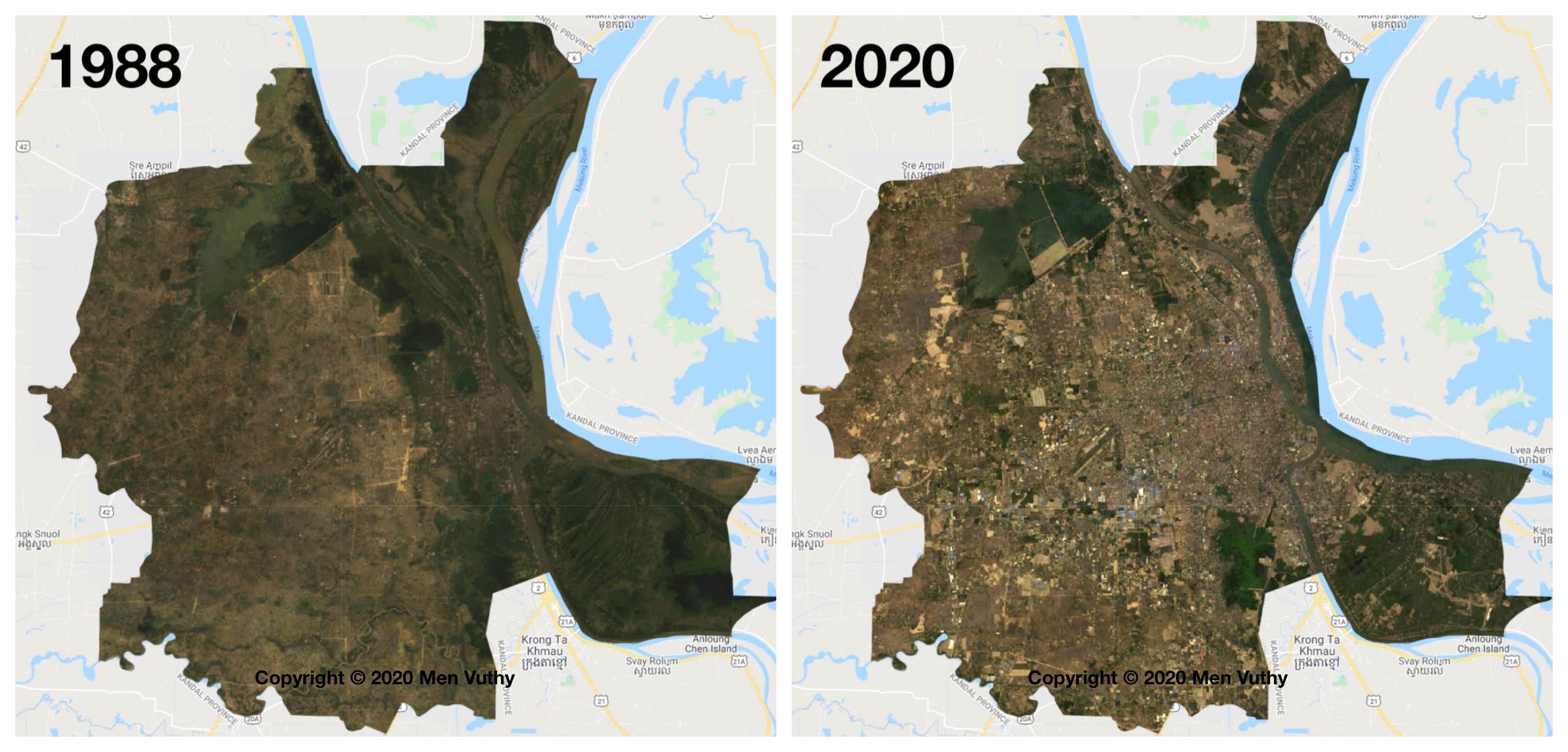
Phnom Penh City: 1988 - 2020
More than thirty years ago, buildings and streets were barely on the map of Phnom Penh city. In 1988 it was home to about 615,000 people; however, 33 years later that had risen to more than 2 million according to worldpopulationreview.com.

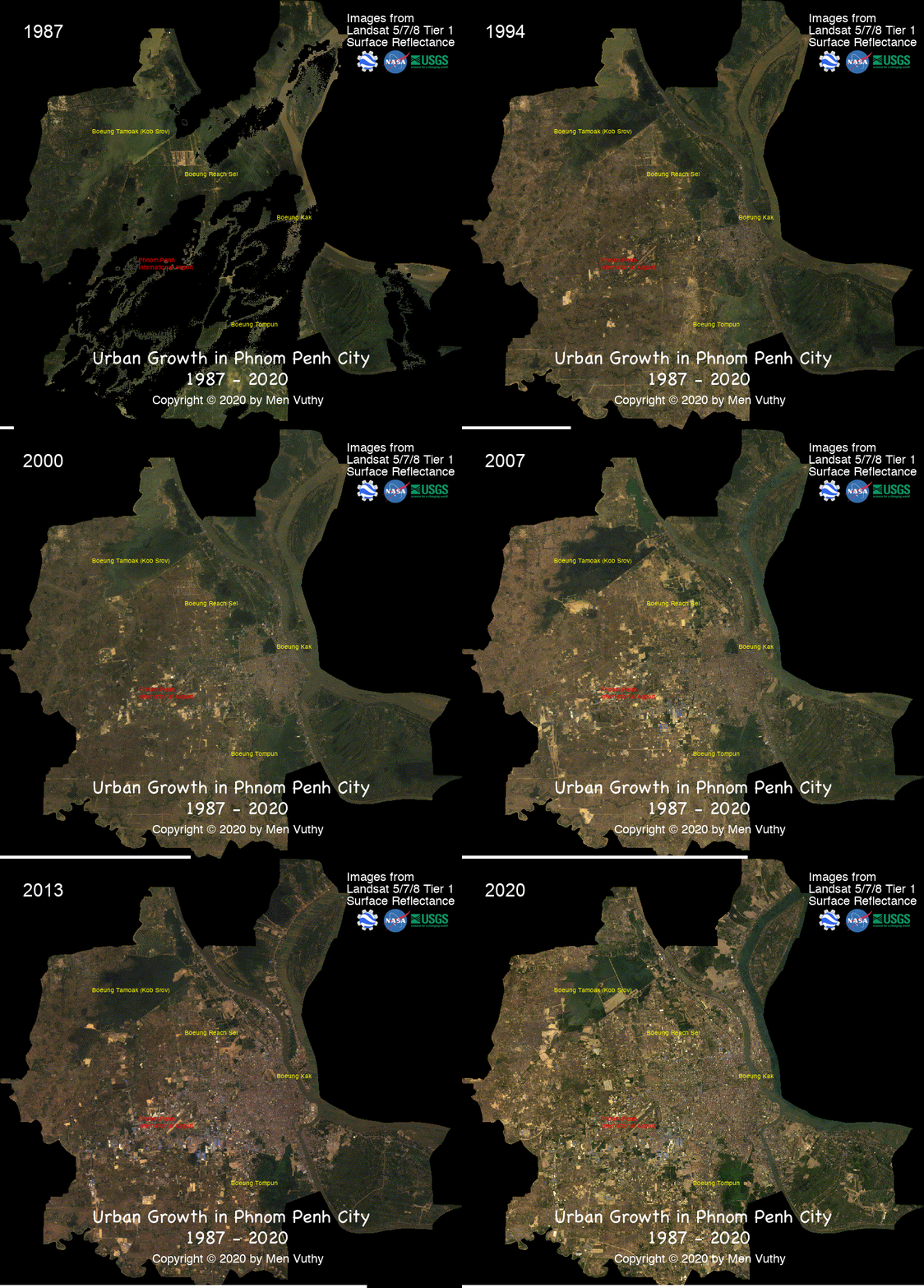
The yearly images were produced from the images of Landsat Satellite 5, 7 and 8 aiming at illustrating the spatial and temporal changes of urban growth in Phnom Penh city from 1988 to 2020.
Here is the Timelapse of Phnom Penh city (1987 - 2020):

Landsat Processing Methods
The development of image for each year was performed in Jupiter Notebook without having to download any image collection from the satellite’s website and resort to any GIS Desktop software. The entire geoprocessing and remote sensing routine requires Earth Engine Python API and geemap. The geemap Python package is built upon the ipyleaflet and folium packages and implements several methods for interacting with Earth Engine data layers, such as Map.addLayer(), Map.setCenter(), and Map.centerObject().
After installation of these packages into your library based on the guideline of geemap, you may follow the main steps below to develop the image:
- Import
geemap packageinto Python - Create an interactive map (Map)
- Add boundary of region of interest (roi) in to Map
- Define a function to mask clouds for Landsat 4, 5, 7 and 8
- Import Landsat image collection based on target year by filtering the date, and roi
- Mask the clouds of the imported image and clip the image within roi
- Add layer of each image following the target year into Map. For viewing, selection of Bands is different following to the type of Landsat Image.
- After receiving the cloudMasked images of each year, composite them into a timelapse imagery in a GIF format or a video based on own’s interest.
Sample Scripts
In this sample script, I raised three years (i.e. 2000, 2010, and 2020) for different Landsat satellite images. As for other years, you modify and add more by yourself following the instruction below.
1. Import geemap package into Python
---
# Installs geemap package
import subprocess
try:
    import geemap
except ImportError:
    print('geemap package not installed. Installing ...')
    subprocess.check_call(["python", '-m', 'pip', 'install', 'geemap'])
# Checks whether this notebook is running on Google Colab
try:
    import google.colab
    import geemap.eefolium as geemap
except:
    import geemap
# Authenticates and initializes Earth Engine
import ee
try:
    ee.Initialize()
except Exception as e:
    ee.Authenticate()
    ee.Initialize()
---
2. Create an interactive map (Map)
---
# Map zooming at Phnom Penh city
Map = geemap.Map(zoom=4)
Map.setCenter(104.8997174646636, 11.555294803579315, 11);
Map
---
3. Add boundary of region of interest (roi) in to Map
In this project, I used shapefile of Phnom Penh boundary as my region of interest.
---
roi = geemap.shp_to_ee('~/PhnomPenh.shp')
Map.addLayer(roi, {}, 'PhnomPenh_Boundary')
---
4. Define a function to mask clouds for Landsat 4, 5, 7 and 8
CloudMask script is available at Earth Engine Data Catalog; however, converting from Java scripts to Python scripts is necessary.
---
# Surface reflectance QA band to mask clouds.
def cloudMaskL457(image):
  qa = image.select('pixel_qa')
  # If the cloud bit (5) is set and the cloud confidence (7) is high
  # or the cloud shadow bit is set (3), then it's a bad pixel.
  cloud = qa.bitwiseAnd(1 << 5) \
          .And(qa.bitwiseAnd(1 << 7)) \
          .Or(qa.bitwiseAnd(1 << 3))
# Remove edge pixels that don't occur in all bands
  mask2 = image.mask().reduce(ee.Reducer.min())
  return image.updateMask(cloud.Not()).updateMask(mask2)
---
5. Import Landsat image collection based on target year
The Landsat satellite images are followed by the year. For instance, Lansat 5 is 1984-2012, Landsat 7 is 1999-present, and Landsat 8 is 2013-present. Further details about each Landsat satellite image is described Here. Therefore, the earlier years can also be found in the image collection of older satellite, too.
---
# Landsat 5, Year: 2000
collection_2000 = ee.ImageCollection('LANDSAT/LT05/C01/T1_SR') \
    .filterDate('2000-01-01', '2000-12-31')\
    .filterBounds(roi)

# Landsat 7, Year: 2010
collection_2010 = ee.ImageCollection('LANDSAT/LE07/C01/T1_SR') \
    .filterDate('2010-01-01', '2010-12-31')\
    .filterBounds(roi)

# Landsat 8, Year: 2020
collection_2020 = ee.ImageCollection('LANDSAT/LC08/C01/T1_SR') \
    .filterDate('2020-01-01', '2020-08-05')\
    .filterBounds(roi)
---
6. Mask the clouds of satellite image and clip within roi
---
# Mask cloud of image in 2000
PP_2000 = collection_2000 \
    .map(cloudMaskL457) \
    .median()\
    .clip(roi)

# Mask cloud of image in 2010
PP_2010 = collection_2010 \
    .map(cloudMaskL457) \
    .median()\
    .clip(roi)

# Mask cloud of image in 2020
PP_2020 = collection_2020 \
    .map(cloudMaskL457) \
    .median()\
    .clip(roi)
---
7. Add layer of each image into interactive Map.
---
# visulization bands for Landsat 5
vis_1 = {
    'bands': ['B3', 'B2', 'B1'], # [Red, Green, Blue]
    'min': 0,
    'max': 4000,
    'gamma': [1, 1, 1]
}

# visulization bands for Landsat 7
vis_2 = {
    'bands': ['B3', 'B2', 'B1'], # [Red, Green, Blue]
    'min': 0,
    'max': 4000,
    'gamma': [1, 1, 1]
}

# visulization bands for Landsat 8
vis_3 = {
    'bands': ['B4', 'B3', 'B2'], # [Red, Green, Blue]
    'min': 0,
    'max': 4000,
    'gamma': [1, 1, 1]
}

# Add layer to Map
Map.addLayer(PP_2000, vis_1, 'Phnom Penh-2000')
Map.addLayer(PP_2010, vis_2, 'Phnom Penh-2010')
Map.addLayer(PP_2020, vis_3, 'Phnom Penh-2020')
---
8. Composite images into a timelapse imagery in a GIF format.
In order to composite images into a timelapse imagery, you need to have a collection of several images following a time frame. Due to different band type for visualization of Landsat satellite, I haven’t found a way to write a single script to make GIF images from each satellite. Therefore, I composite the images from each satellite separately. For example, a composite of image collection from Landsat 5, a composite of image collection from Landsat 7, and a composite of image collection from Landsat 8. In the sample script above, there are only three years. Given that, there’s no need to composite these three images in Python. You can make it manually by using online or computer application.
However, you may use the below script in case you have more years of images from different Landsat satellite.
---
# Composite all images into a collection
PhnomPenh987to013 = ee.ImageCollection([PP_1987,PP_1988, PP_1989,PP_1990,PP_1991,PP_1992,
                                      PP_1993,PP_1994,PP_1995,PP_1996,PP_1997,PP_1998,PP_1999,PP_2000,
                                      PP_2001,PP_2002,PP_2003,PP_2004,PP_2005,PP_2006,PP_2007,PP_2008,
                                      PP_2009,PP_2010,PP_2011,PP_2012,PP_2013])
# visulization bands for Landsat 5 and 7
video_args1 = {
  'dimensions': 768,
  'region': roi,
  'framesPerSecond': 1,
  'bands': ['B3', 'B2', 'B1'],
  'min': 0,
  'max': 4000,
  'gamma': [1, 1, 1]
}

# Export image
import os
work_dir = os.path.join(os.path.expanduser('~/Result')) # Set path for saving folder
out_gif = os.path.join(work_dir, "PP_to2013.gif") # Save file as
geemap.download_ee_video(PhnomPenh987to013, video_args1, out_gif) # Creating GIF

# Composite all images into a collection
PhnomPenh14to20 = ee.ImageCollection([PP_2014,PP_2015,PP_2016,PP_2017,PP_2018,PP_2019,PP_2020])
# visulization bands for Landsat 8
video_args = {
  'dimensions': 768,
  'region': roi,
  'framesPerSecond': 1,
  'bands': ['B4', 'B3', 'B2'],
  'min': 0,
  'max': 4000,
  'gamma': [1, 1, 1]
}

# Export image
import os
work_dir = os.path.join(os.path.expanduser('~/Result'))
out_gif = os.path.join(work_dir, "PhnomPenh14to20.gif")
geemap.download_ee_video(PhnomPenh14to20, video_args, out_gif)
---
Timelapse Video
That’s all, everyone !
That’s it for this piece of work! We have successfully implemented classic geoprocessing and remote sensing workflows without having to use ArcGIS or QGIS. For the whole workflow, you may contact me directly. If you have questions or suggestions especially on the problem I couldn’t solve above, please feel free to let me know.
Cheers,
Vuthy
Source code is available at: GitHub


