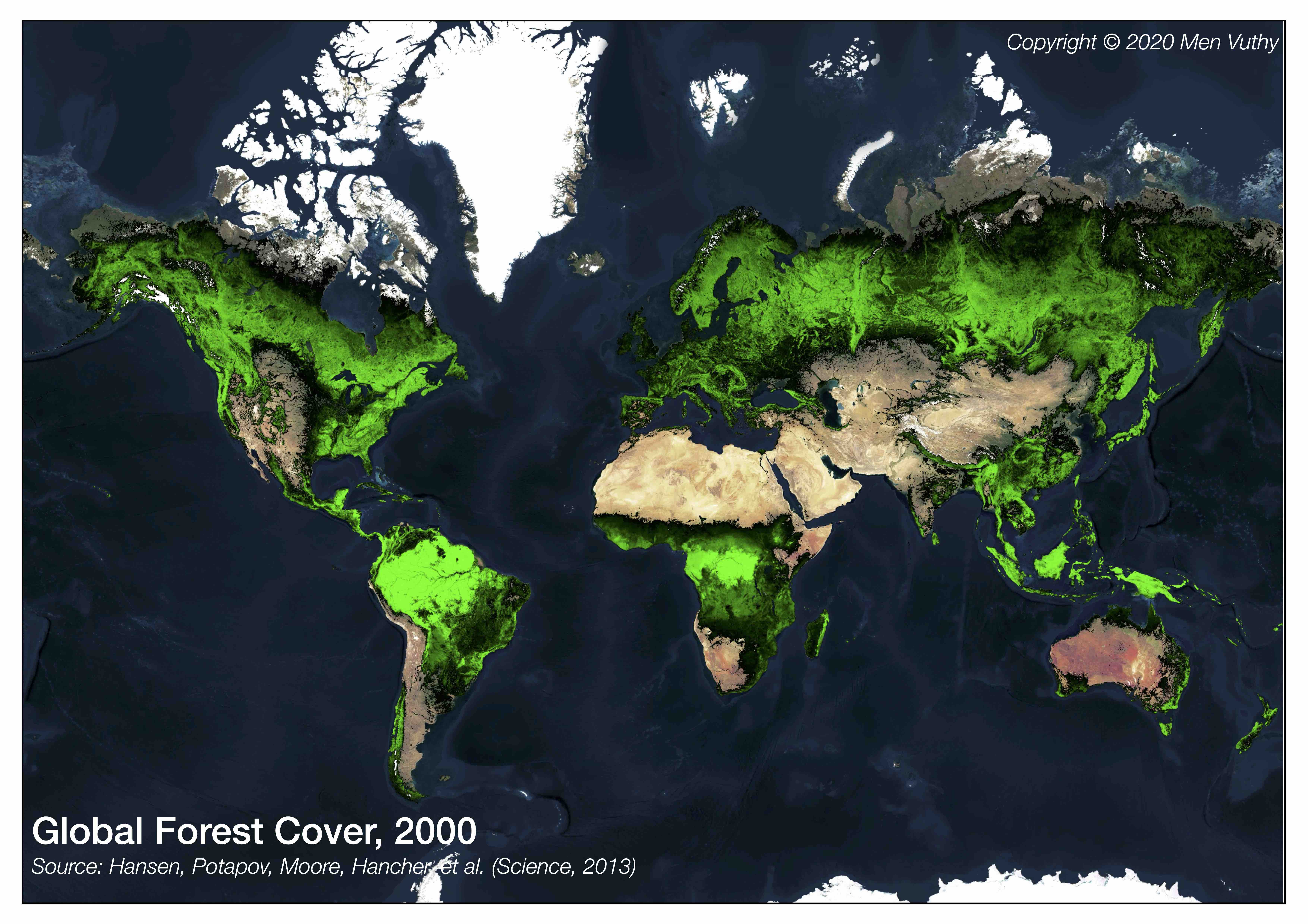
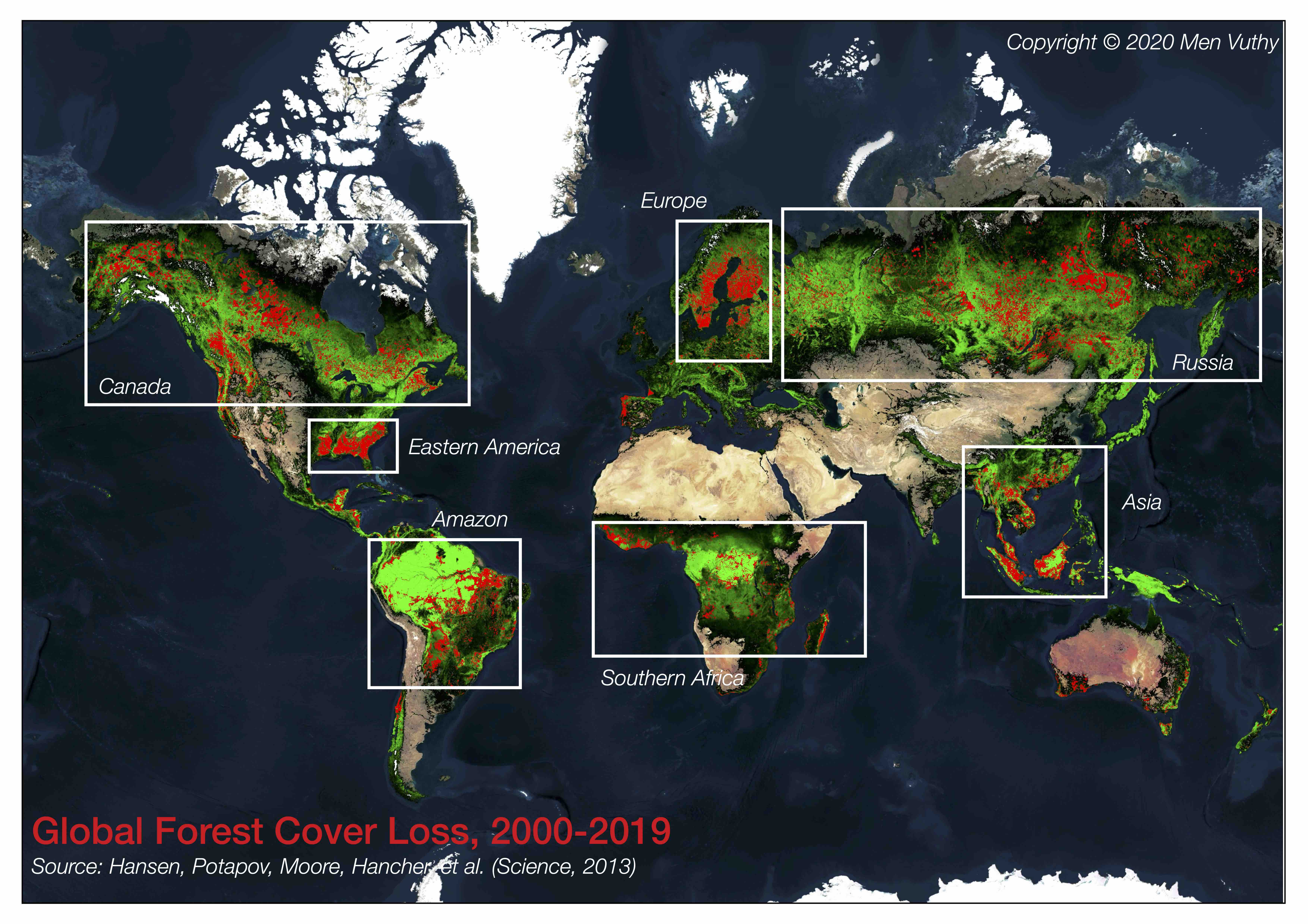
Forest cover plays an essential role in delivering important ecosystem services, including biodiversity richness, climate regulation, carbon storage, and water supplies (1). However, spatially and temporally detailed information on global-scale forest cover changes at a high resolution did not exist until M.C. Hansen and his team in the University of Maryland, USA developed a global-scale forest change and published the works in 2013 (2). Hansen et al. 2013 (2) mapped global tree cover extent, loss, and gain annually for the period from 2000 to 2012 from Landsat imagery at a spatial resolution of 30 m, especially the datasets have been updated every year.
The data source of information content presented here is publicly availble for both download and web-based visualizations. However, downloading and processing such a large dataset are extremely tedious, and extracting it for analysis on a cloud platform can be the main challenges for some engineers and scientists who are struggling with remote sensing technology. Therefore, here I will illustrate one of many remote sensing methods to extract the datasets to:
- Visualize the global forest cover in 2000, and forest cover loss during the period 2000-2019.
- Examine the spatial and temporal changes of both forest cover loss and gain in Cambodia from 2000 to 2019.
- Compute the yearly forest cover and loss in Cambodia from 2000 to 2019.
Primary Notice: These dataset illustration and visualization are aimed for Education Purpose only.
Global Forest Cover and Loss
In this dataset, there are four important definitions as following:
- Trees are defined as vegetation taller than 5m in height and are expressed as a percentage per output grid cell.
- Forest Cover Loss is defined as a stand-replacement disturbance, or a change from a forest to non-forest state, during the period 2000–2019.
- Forest Cover Gain is defined as the inverse of loss, or a non-forest to forest change entirely within the period 2000–2012.
- Forest Loss Year is a disaggregation of total ‘Forest Loss’ to annual time scales.
Forest Cover Loss and Gain in Cambodia
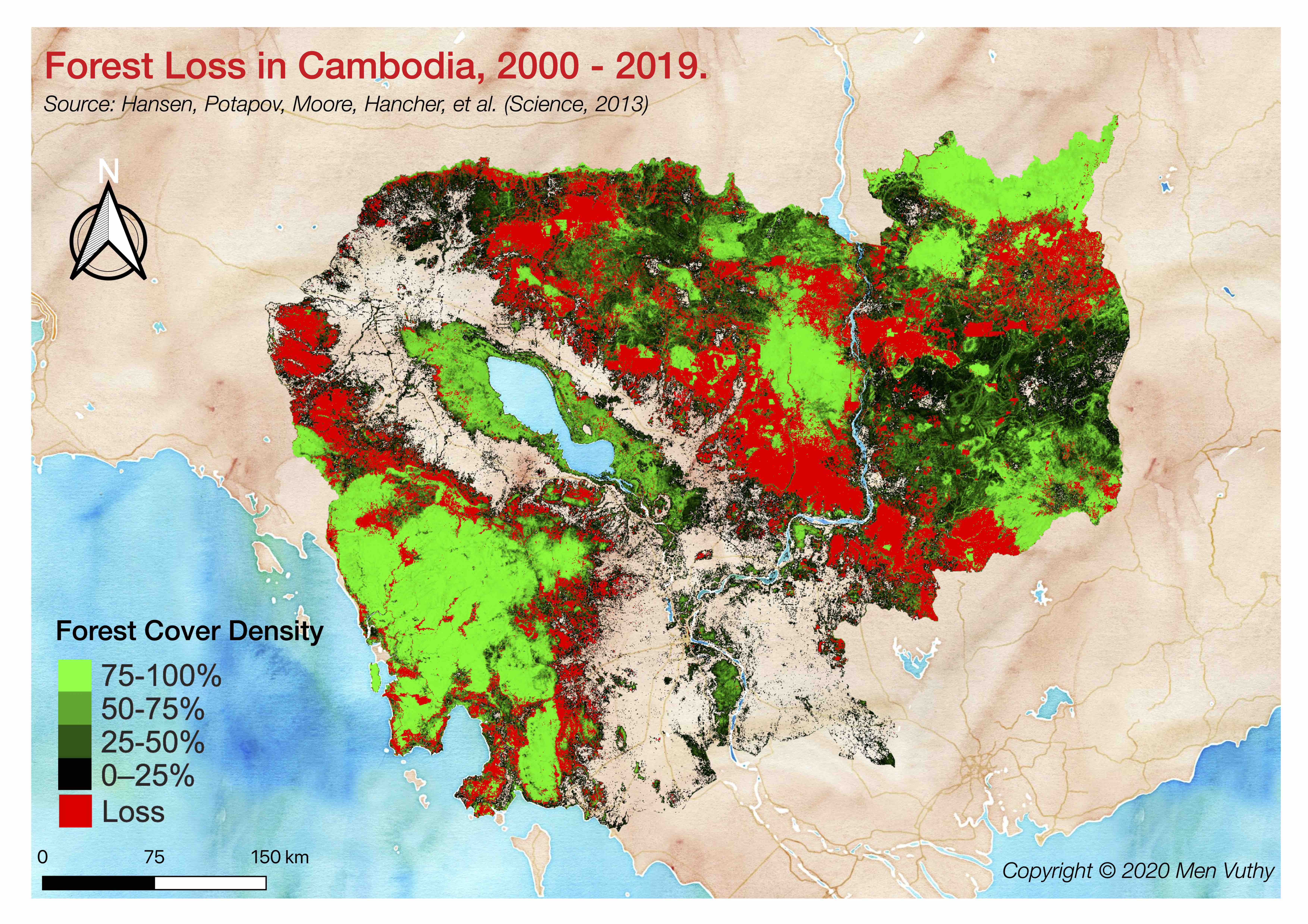
- Forest Cover Loss
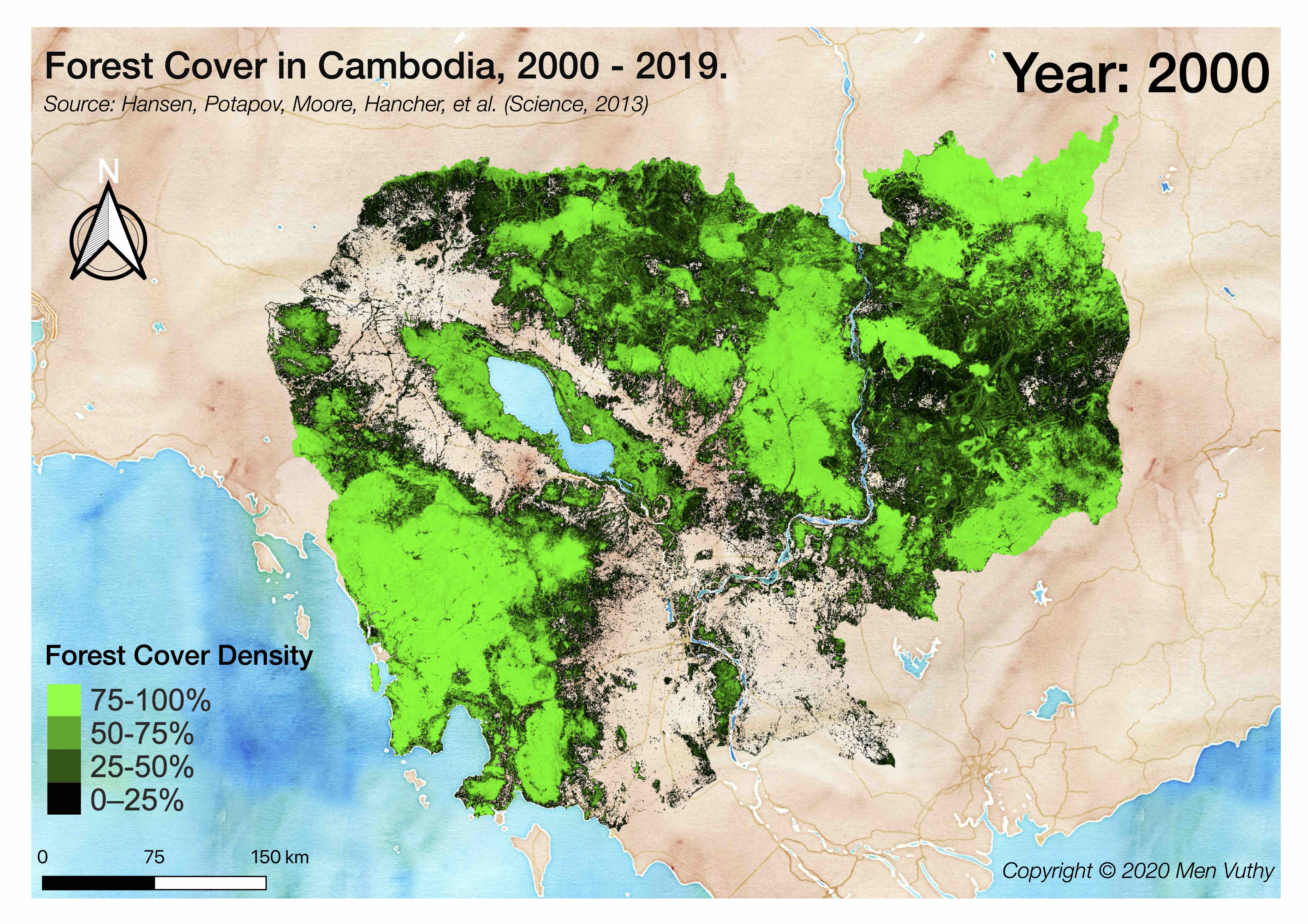
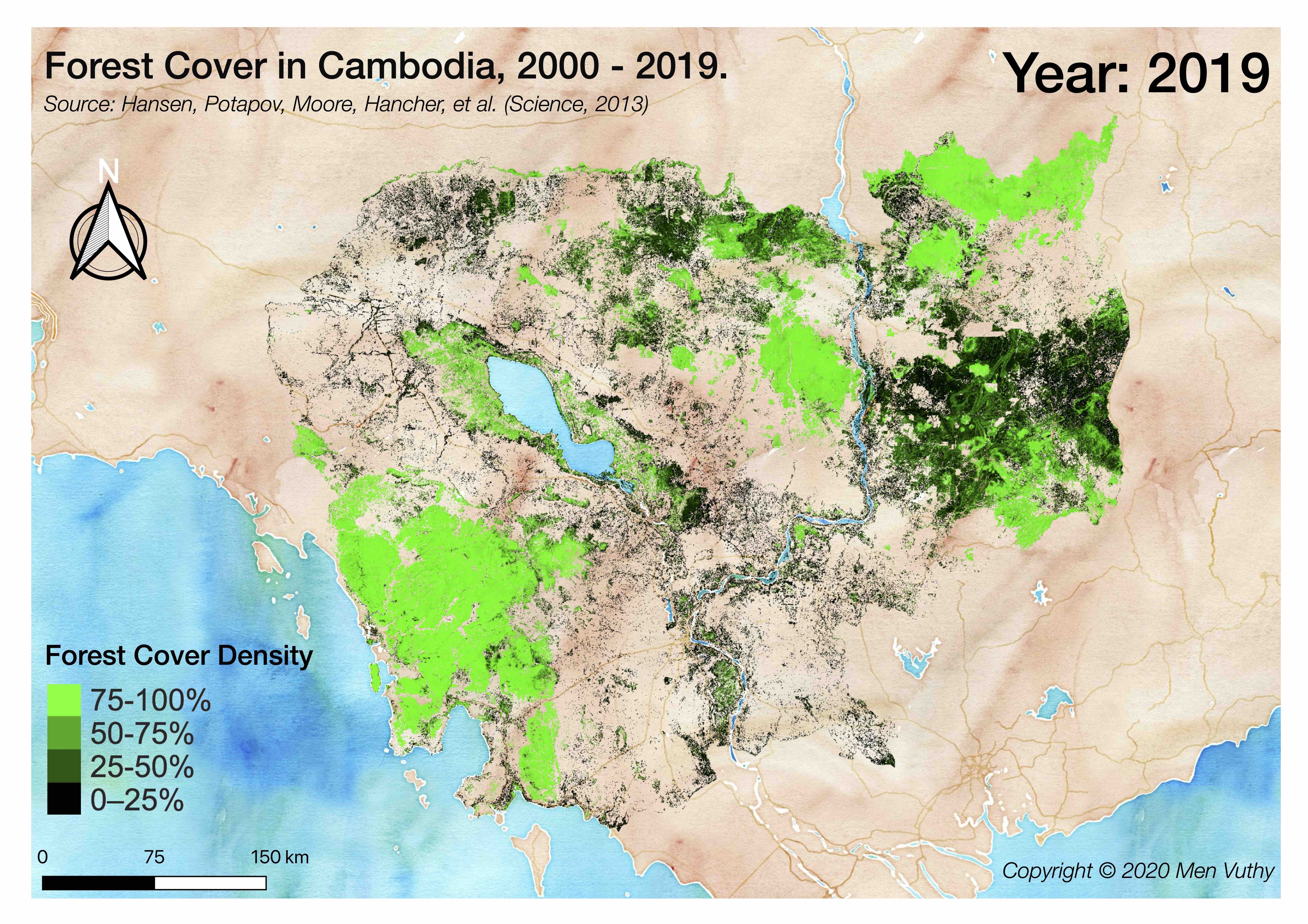
Figure 2 shows the comparison image of forest cover between 2000 and 2019 of the whole country.
Video showing spatial and temporal changes of forest cover in Cambodia from 2000 to 2019.
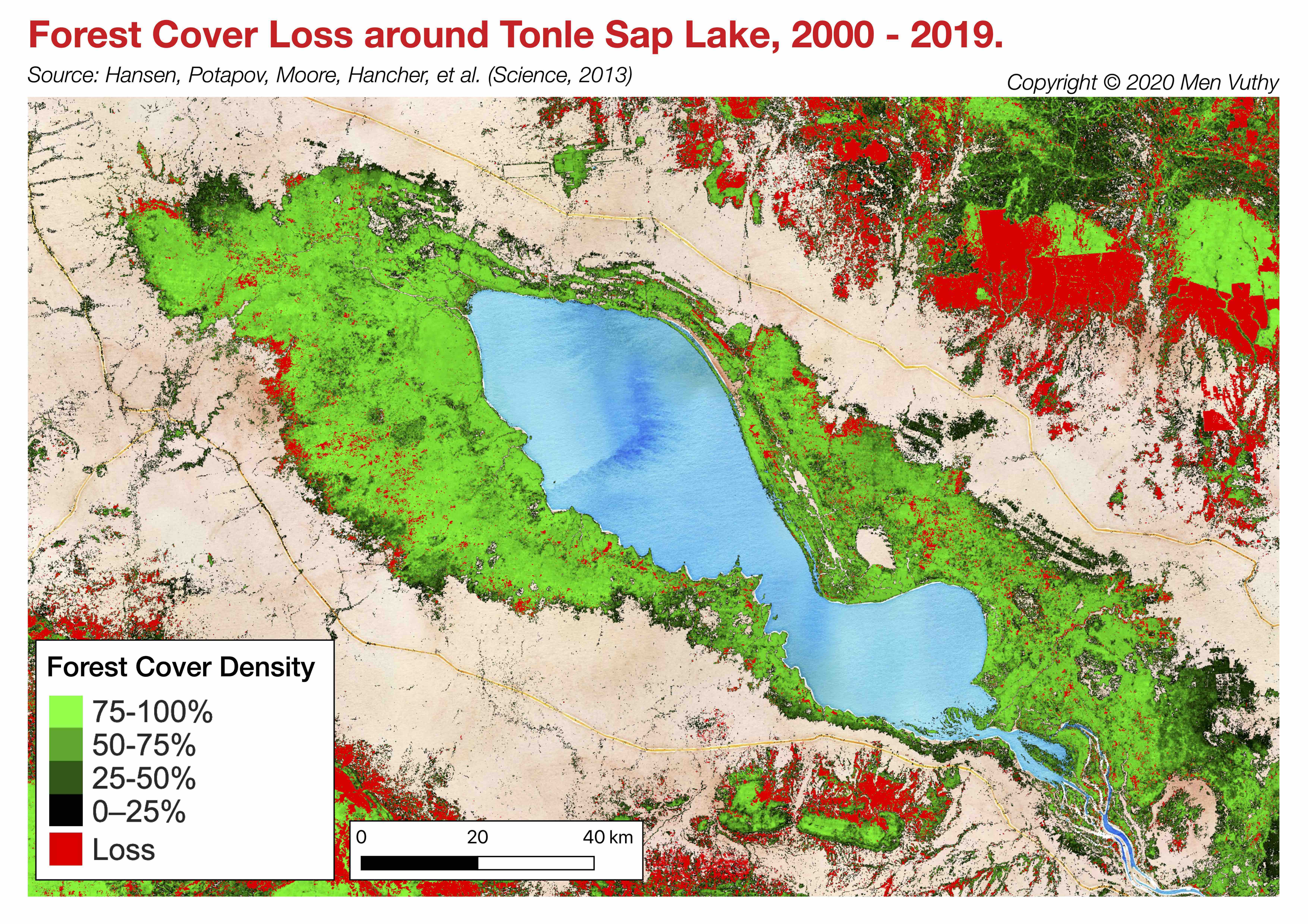
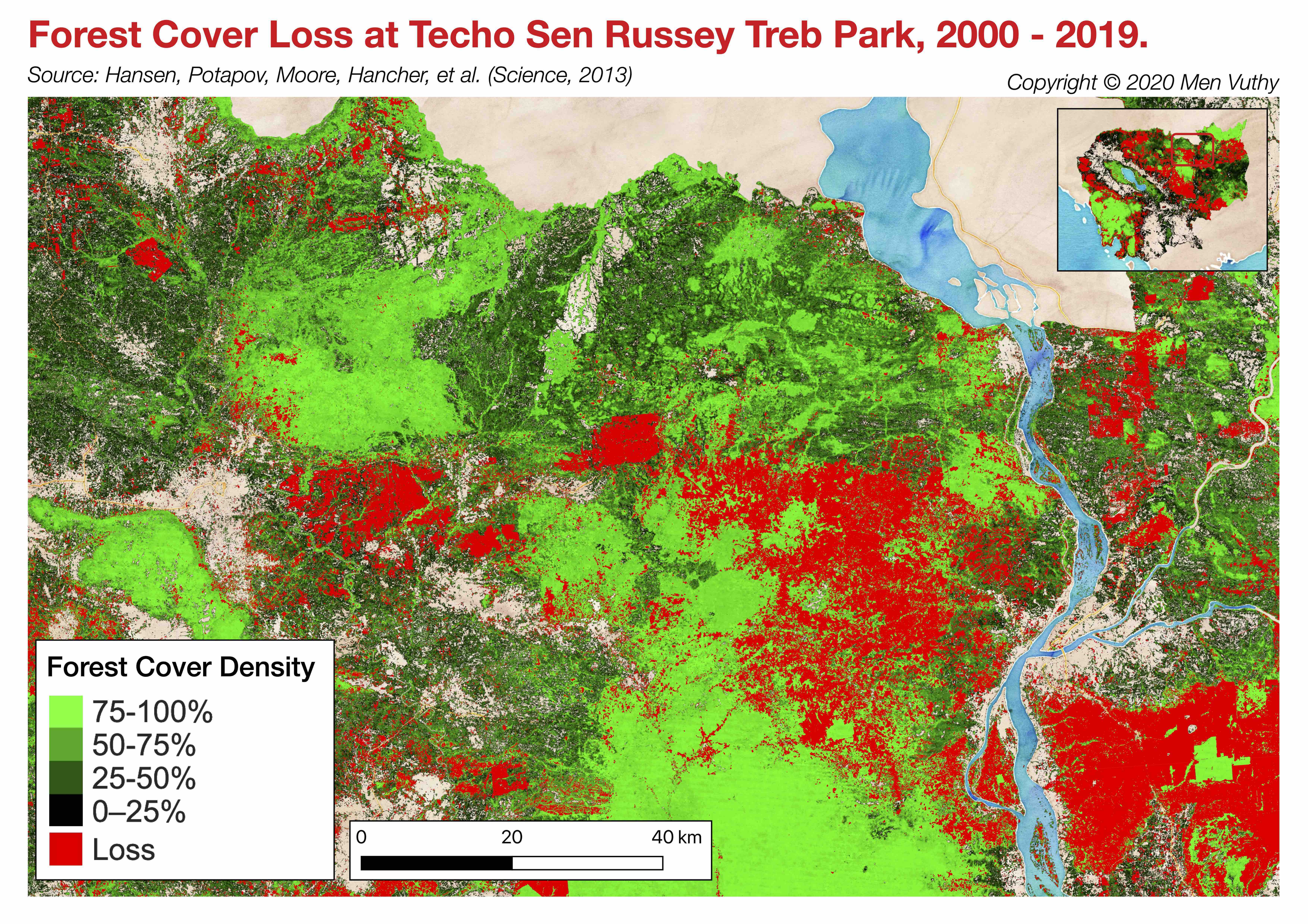
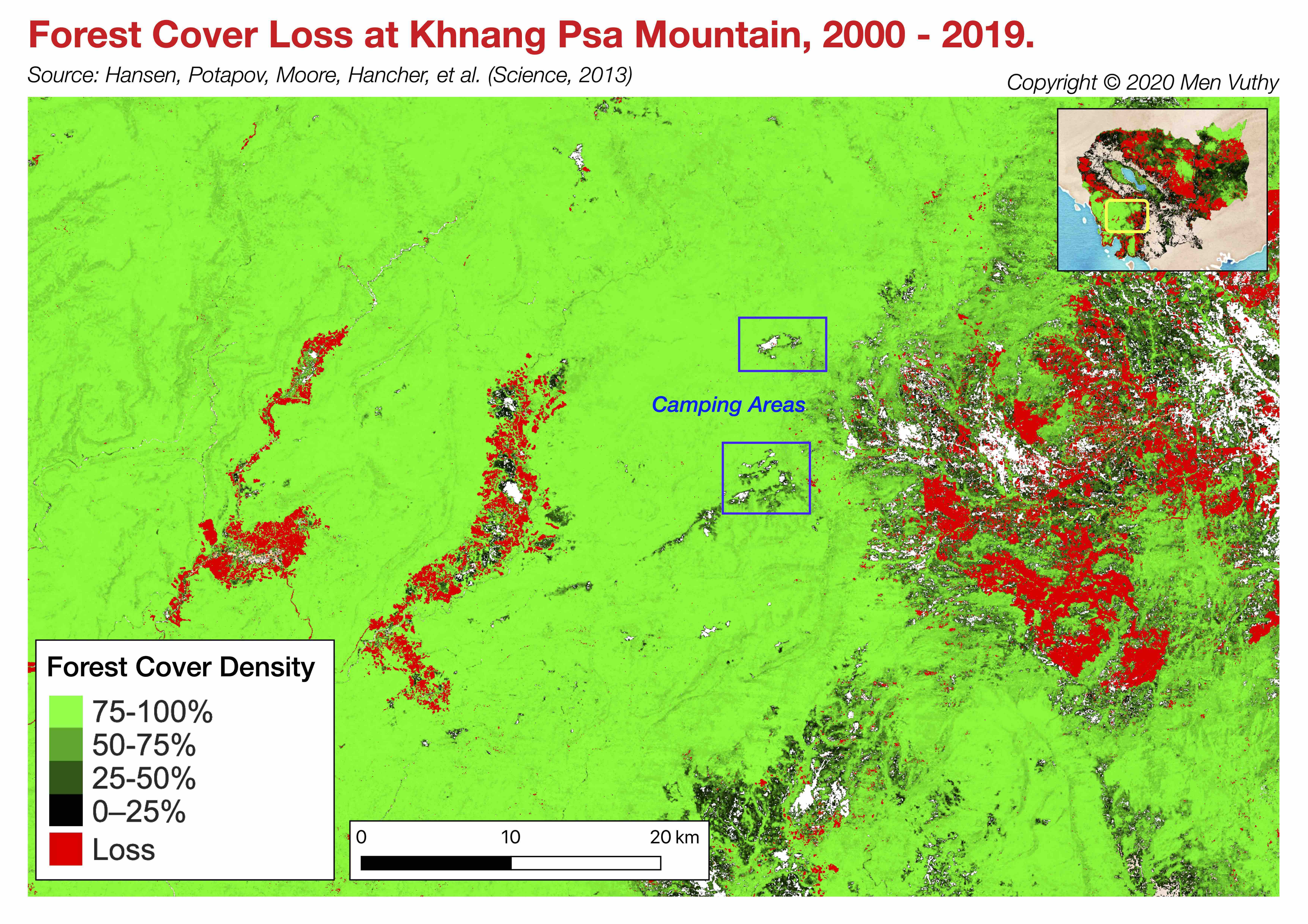
By only viewing the video, the forest cover loss of some areas are exaggerated due to the far view of image and also the low density of forest canopy at those areas; hence, it is important to zoom into some specific areas to have a closer view of the forest cover and loss. Figure 3 are the images of some well-known areas in Cambodia which provide a clearer and closer look on forest cover and loss.
- Forest Cover Gain
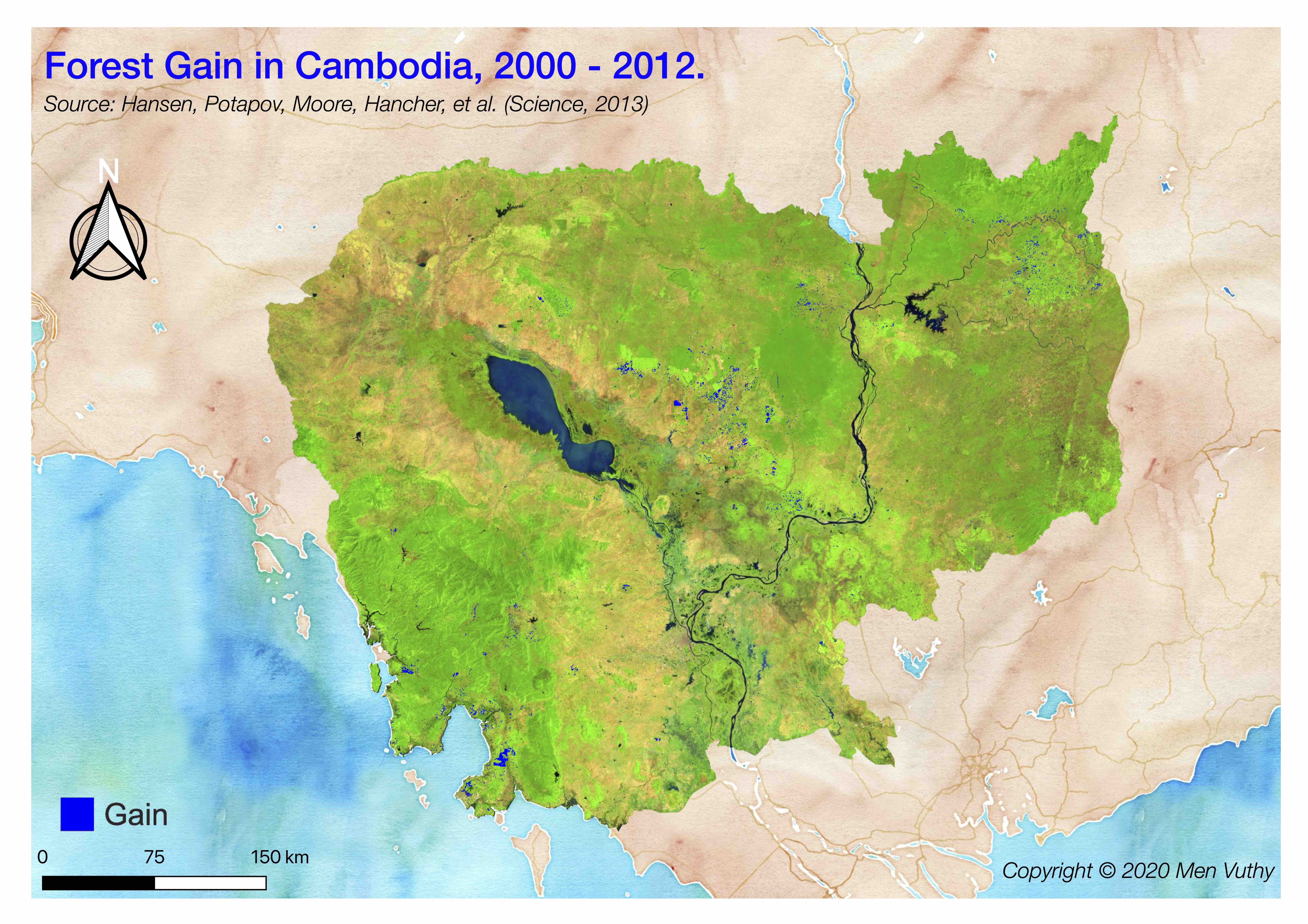
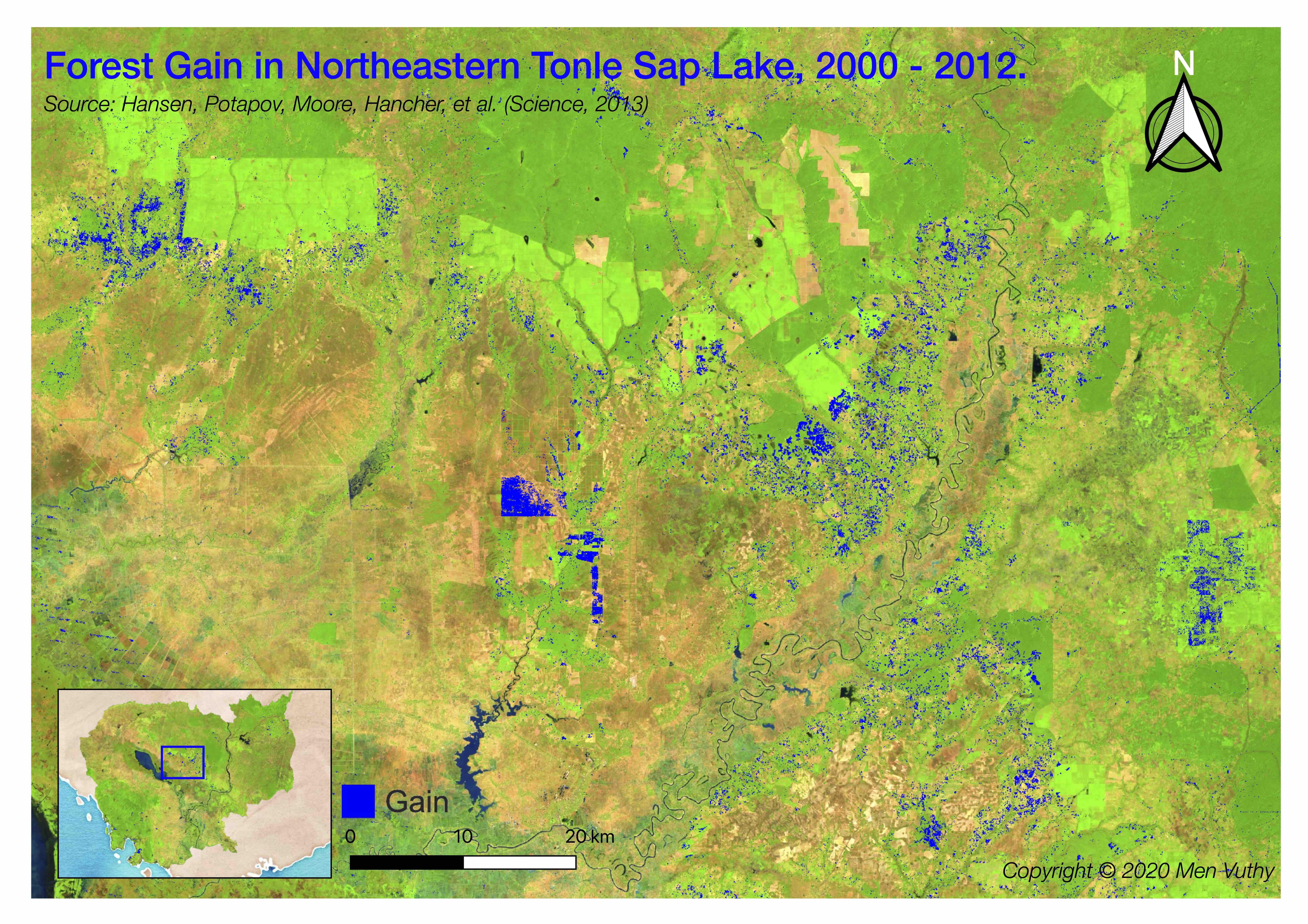
Figure 4 shows the image of forest gain between 2000 and 2012 of the whole Cambodia and Northeastern Tonle Sap Lake area.
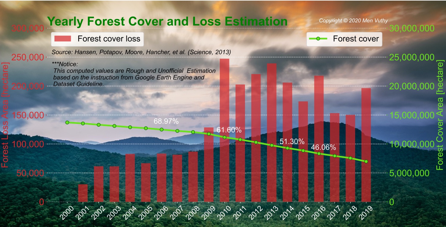
Yearly Forest Cover and Loss in Cambodia
Forest loss was defined as a stand-replacement disturbance or the complete removal of tree cover canopy at the Landsat pixel scale (2). The estimation yearly forest cover and loss are shown in figures below (Figure 5):
Warning Notice: All computed values here are the rough and unofficial calculation based on the instruction from Google Earth Engine. The user should be concerned of the accuracy with the actual data in their region of interest and the comparison with the official data source.
Methodology
Extraction, computation and visualization of Hansen et al. 2013 (2) global forest cover data in this work are performed on cloud platform with the help of QGIS, Python, and Google Earth Engine. Therefore, it is important to equip with some background on programming language and QGIS application. Below, I will instruct how to extract, visualize, and compute the global forest cover data, and Cambodia will be chosen as a case study.
1. Extraction and Visualization of Global Forest Cover and Loss
There are many methods to extract and visulaize the remote sensing dataset, for example, by using Earth Engine JavaScript API. Under this purpose, it is, however, conducted in QGIS since the performace and loading speed of interactive maps are better. In order to connect QGIS with the earth engine datasets, installation of Google Earth Engine Plugin is first necessary. After that, open the Python Console in QGIS, and the global forest cover data will appear by running the script I provide here with the short description written with the hashtag (#) sign.
---
# Import module
import ee
from ee_plugin import Map

# Add Earth Engine dataset
image = ee.Image('UMD/hansen/global_forest_change_2019_v1_7')
forest = image.select(['treecover2000'])
loss = image.select(['loss'])
lossYear = image.select(['lossyear'])

# visualization setting
vis = {
'min': 0,
'max': 100,
'palette': ['#000000', '#005500', '#00AB00', '#00FF00']
}

# Add layer by masking the unecessary pixels from the map
Map.addLayer(forest.updateMask(forest), vis , 'Global Forest in 2000')
Map.addLayer(loss.updateMask(loss), {'palette': ['#FF0000']} , 'Loss 2000-2019')
---
2. Examination of Forest Cover Loss and Gain in Cambodia
In order to target to any area, the boundary feature must be given so that the dataset will be clipped and shown for that feature only. In this example, Cambodia boundary was extracted from Large Scale International Boundary (LSIB) dataset provided by the United States Office of the Geographer. After setting the boundary of Cambodia, the forest cover loss and gain can be shown by running the script below. Besides QGIS, it can also be done in Google Earth Engine based on the instruction on Quantifying Forest Change; however, it may be a bit challenging when it comes to downloading the data from cloud to local storage for analyzing or mapping.
---
import ee
from ee_plugin import Map

countries = ee.FeatureCollection('USDOS/LSIB_SIMPLE/2017')
# // Get a feature collection with just the Cambodia feature.
roi = countries.filter(ee.Filter.eq('country_co', 'CB'))

# Add Landsat 8 Imagery for the year 2000 and 2019
L8_2000 = ee.ImageCollection('LANDSAT/LT05/C01/T1_SR') \
    .filterDate('2000-01-01', '2000-12-31')\
    .filterBounds(roi)
L8_2019 = ee.ImageCollection('LANDSAT/LC08/C01/T1_SR') \
    .filterDate('2019-01-01', '2019-12-31')\
    .filterBounds(roi)

# Define CloudMask Function
def cloudMaskL457(image):
  qa = image.select('pixel_qa')
  # If the cloud bit (5) is set and the cloud confidence (7) is high
  # or the cloud shadow bit is set (3), then it's a bad pixel.
  cloud = qa.bitwiseAnd(1 << 5) \
          .And(qa.bitwiseAnd(1 << 7)) \
          .Or(qa.bitwiseAnd(1 << 3))
  # Remove edge pixels that don't occur in all bands
  mask2 = image.mask().reduce(ee.Reducer.min())
  return image.updateMask(cloud.Not()).updateMask(mask2)

CB_2000 = L8_2000 \
    .map(cloudMaskL457) \
    .median()\
    .clip(roi)
CB_2019 = L8_2019 \
    .map(cloudMaskL457) \
    .median()\
    .clip(roi)

# visualization setting
vis_1 = {
    'bands': ['B5', 'B4', 'B3'],
    'min': 0,
    'max': 4000,
    'gamma': [1, 1, 1]
}
vis_2 = {
    'bands': ['B6', 'B5', 'B4'],
    'min': 0,
    'max': 4000,
    'gamma': [1, 1, 1]
}

Map.addLayer(CB_2000, vis_1, 'CB_2000')
Map.addLayer(CB_2019, vis_2, 'CB_2019')

# Add Earth Engine dataset
image = ee.Image('UMD/hansen/global_forest_change_2019_v1_7').clip(roi)
treeCover = image.select(['treecover2000'])
lossImage = image.select(['loss'])
gainImage = image.select(['gain'])

# visualization setting
vis = {
'min': 0,
'max': 100,
'palette': ['#000000', '#005500', '#00AB00', '#00FF00']
}

# Add the tree cover layer in green.
Map.addLayer(treeCover.updateMask(treeCover), vis , 'Forest in 2000')

# Add the loss layer in red.
Map.addLayer(lossImage.updateMask(lossImage),{'palette': ['FF0000']}, 'Loss')

# Add the gain layer in blue.
Map.addLayer(gainImage.updateMask(gainImage),{'palette': ['0000FF']}, 'Gain')
---
As for creating yearly forest cover map, the following script was written based on the data instruction on Image Calculation. Here is the script for creating the images of each year:
---
import ee
from ee_plugin import Map

countries = ee.FeatureCollection('USDOS/LSIB_SIMPLE/2017')
roi = countries.filter(ee.Filter.eq('country_co', 'CB'))

image = ee.Image('UMD/hansen/global_forest_change_2019_v1_7').clip(roi)
forest = image.select(['treecover2000'])
loss = image.select(['loss'])
lossYear = image.select(['lossyear'])

#2001
lossInFirst1 = lossYear.gte(1).And(lossYear.lte(1))
forestAt2001 = forest.where(lossInFirst1.eq(1), 0)
#2002
lossInFirst2 = lossYear.gte(1).And(lossYear.lte(2))
forestAt2002 = forest.where(lossInFirst2.eq(1), 0)
.
.
.

#2019
lossInFirst19= lossYear.gte(1).And(lossYear.lte(19))
forestAt2019 = forest.where(lossInFirst19.eq(1), 0)

vis = {
'min': 0,
'max': 100,
'palette': ['#000000', '#005500', '#00AB00', '#00FF00']
}

Map.addLayer(forestAt2001.updateMask(forestAt2001), vis, 'Forest in 2001')
.
.
.
Map.addLayer(forestAt2019.updateMask(forestAt2019), vis, 'Forest in 2019')
---
3. Computation of Yearly Forest Loss in Cambodia
The computation for yearly forest cover and loss are conducted both in Earth Engine Code Editor and Python in Jupiter Notebook. Based on the instruction on how to quantify the yearly forest loss in the GEE guideline, the yearly forest loss in Cambodia can be estimated by changing the region of interest of the provided script. Regarding the detail estimation method, please carefully read the guideline of dataset usage.
Here is the script to run in GEE Code Editor for calculating yearly forest loss in Cambodia:
---
// Load country boundaries from LSIB.
var countries = ee.FeatureCollection('USDOS/LSIB_SIMPLE/2017');
// Get a feature collection with just the Congo feature.
var cambo = countries.filter(ee.Filter.eq('country_co', 'CB'));
Map.addLayer(cambo, {}, 'Cambodia')

// Get the loss image.
// This dataset is updated yearly, so we get the latest version.
var gfc2017 = ee.Image('UMD/hansen/global_forest_change_2019_v1_7');
var lossImage = gfc2017.select(['loss']);
var lossAreaImage = lossImage.multiply(ee.Image.pixelArea());

var lossYear = gfc2017.select(['lossyear']);
var lossByYear = lossAreaImage.addBands(lossYear).reduceRegion({
  reducer: ee.Reducer.sum().group({
    groupField: 1
    }),
  geometry: cambo,
  scale: 30,
  maxPixels: 1e9
});
print(lossByYear);

var statsFormatted = ee.List(lossByYear.get('groups'))
  .map(function(el) {
    var d = ee.Dictionary(el);
    return [ee.Number(d.get('group')).format("20%02d"), d.get('sum')];
  });
var statsDictionary = ee.Dictionary(statsFormatted.flatten());
print(statsDictionary);

var chart = ui.Chart.array.values({
  array: statsDictionary.values(),
  axis: 0,
  xLabels: statsDictionary.keys()
}).setChartType('ColumnChart')
  .setOptions({
    title: 'Yearly Forest Loss',
    hAxis: {title: 'Year', format: '####'},
    vAxis: {title: 'Area (square meters)'},
    legend: { position: "none" },
    lineWidth: 1,
    pointSize: 3
  });
print(chart);
---
In order to calculate yearly forest cover, zonal_statistics_by_group function in geemap module was used in Python Jupyter Notebook to sum all forest cover pixels based on the size and forest canopy density of each pixel. Before calculation, installation of geemap package may be necessary at the beginning if it is not yet installed on PC. The installation instruction is available here.
To run the script below, the script in section 2 about creating yearly forest cover map should be firstly run in Jupyter Notebook by just omitting “from ee_plugin import Map” and import some other modules as following:
---
# Installs geemap package
import subprocess

try:
    import geemap
except ImportError:
    print('geemap package not installed. Installing ...')
    subprocess.check_call(["python", '-m', 'pip', 'install', 'geemap'])

# Checks whether this notebook is running on Google Colab
try:
    import google.colab
    import geemap.eefolium as geemap
except:
    import geemap

# Authenticates and initializes Earth Engine
import ee

try:
    ee.Initialize()
except Exception as e:
    ee.Authenticate()
    ee.Initialize()
import os

[*** Script from Section 2...]

# determine the output folder
out_dir = os.path.join(os.path.expanduser('~'), 'Downloads')

# statistics_type can be either 'SUM' or 'PERCENTAGE'
# denominator can be used to convert square meters to other areal units, such as square kilimeters or hectare
forest_cover = os.path.join(out_dir, 'forest-cover-2001.csv')
geemap.zonal_statistics_by_group(forestAt2001.updateMask(forestAt2001), roi, forest_cover, statistics_type='SUM', denominator=10000, decimal_places=2)

forest_cover = os.path.join(out_dir, 'forest-cover-2002.csv')
geemap.zonal_statistics_by_group(forestAt2002.updateMask(forestAt2002), roi, forest_cover, statistics_type='SUM', denominator=10000, decimal_places=2)
.
.
.
forest_cover = os.path.join(out_dir, 'forest-cover-2019.csv')
geemap.zonal_statistics_by_group(forestAt2019.updateMask(forestAt2019), roi, forest_cover, statistics_type='SUM', denominator=10000, decimal_places=2)
---
That’s all, everyone !
That’s it for this piece of work! I hope this instruction can be useful for engineering student or young professional who may need this lesson to work on their project. For the whole workflow, you may contact me directly. If you have questions or suggestions, please feel free to let me know.
Cheers,
Vuthy
Reference
- Foley, Jonathan A., et al. “Global consequences of land use.” science 309.5734 (2005): 570-574.
- Hansen, Matthew C., et al. “High-resolution global maps of 21st-century forest cover change.” science 342.6160 (2013): 850-853.
Related websites
- Global Forest Change 2000–2019 Data Download
- Introduction to Hansen et al. Global Forest Change Data
- Geemap Package Documentation
- API Tutorial: Hansen/UMD/Google Global Forest Change
Source code is available at: GitHub